Ham radio hobbyists, as the former term indicate, have been all over the time great technicians, but with exceptions, never professionals on electrical or electronics works and related fields.

There are aspects of the radio where the hobbyists rub the professional turf. One of this aspects is antenna design. Until present, the biggest difference between a professional and a hobbyist was the amount of technology available to them, especially measurement equipment. General knowledge was already at hand, as books and encyclopaedias were available to both.

More in depth on antenna design, both professionals and hobbyist manage similar concepts, like SWR (stationary wave relationship), capacitance or inductance of circuits.

Nowadays, it’s easy to see a professional using expensive equipment, mostly software based, performing complex calculations, but, there was a point in time where those calculations were done manually using simple tools like a Smith Chart.

A bit of history

Smith charts were originally developed around 1940 by Phillip Smith as a useful tool for making the equations involved in transmission lines easier to manipulate. With modern computers and the use of software, the Smith chart is no longer used for the calculation of transmission line equations, however, their value in visualising the impedance of an antenna, or a transmission line, has not decreased.

The Smith chart is a graphical calculator, or nomogram, designed for electrical and electronics engineers specialising in radio frequency (RF) engineering to assist in solving problems with transmission lines and matching circuits. The use of the Smith chart, and the interpretation of the results obtained using it, requires a good understanding of AC circuit theory and transmission-line theory, both of which are prerequisites for RF engineers and, why not, for general radio hobbyists.

The Smith chart is a fantastic tool for visualising the impedance of a transmission line and antenna system as a function of frequency. Smith charts can be used to increase understanding of transmission lines and how they behave from an impedance viewpoint. Smith charts are also extremely helpful for impedance matching. The Smith chart is used to display an actual (physical) antenna’s impedance when measured on a Vector Network Analyser (VNA).

Network Analysers

In general, a network analyser is an instrument that measures the parameters of electrical networks. Analysers could be of two main types, Scalar Network Analyser (SNA), that measures amplitude properties only, and Vector Network Analyser (VNA), that measures both amplitude and phase properties.

A Vector Network Analyser (VNA) is a form of RF network analyser widely used for RF design applications. A VNA may also be called a gain–phase meter or an automatic network analyser. An SNA is functionally identical to a spectrum analyser in combination with a tracking generator.

Nowadays, VNAs are the most common type of network analysers, and so references to an unqualified “network analyser” most often mean a VNA.

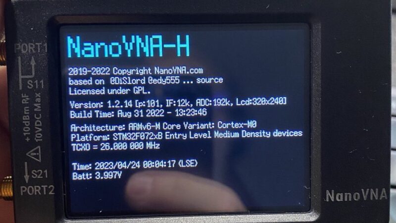
With the advent of software and the cost reduction on materials crafted on China, entry-level devices and do-it-yourself projects have also been available, some for less than $100, mainly from the amateur radio sector. Although these have significantly reduced features compared to professional devices and offer only a limited range of functions, they are often sufficient for private users, especially during studies and for hobby applications up to the single-digit GHz range.

S-Parameters (scattering parameters)

Scattering parameters, or S-parameters, are popular in RF/Microwave circuit design and testing. Following are scattering parameters used for measuring/characterising an RF device.

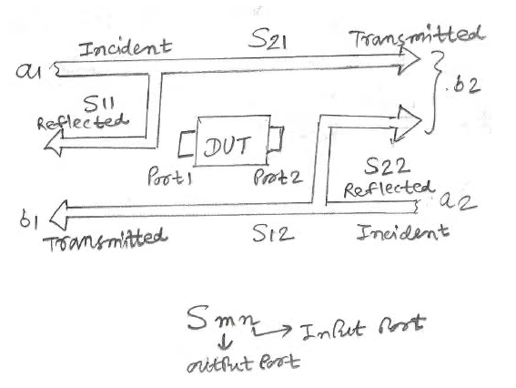
From the Figure 1, beside, following two equations are derived:

b1 = S11 x a1 + S12 x a2 b2 = S21 x a1 + S22 x a2

S11 → Reflection coefficient at Port1 S22 → Reflection coefficient at Port2 S12 → Isolation (Reverse) S21 → Insertion loss (passive device case)

S-parameters are vector entities which are derived from vector based measurements like magnitude or phase. Following scalar measurements are derived from S-parameters:

• Reflection and incident waves (S-parameters S11 & S22):
  • Input SWR
  • Return Loss
  • VSWR
  • Input / output impedance
  • Reflection coefficient
• Transmission and incident waves (S-parameters S21 & S12):
  • Gain / Insertion Loss
  • Isolation
  • Insertion phase
  • Group delay
  • Transmission coefficient

As you can see, S-parameters describe the input-output relationship between ports (or terminals) in an electrical system. For example, if we have 2 ports (intelligently called Port 1 and Port 2), then:

• S12 represents the power transferred from Port 2 to Port 1.
• S21 represents the power transferred from Port 1 to Port 2.

In general, S_nm_ represents the power transferred from Port m to Port n in a multi-port network. These S-parameters are defined in terms of incident and reflected travelling waves.

As it was argued above, a port can be loosely defined as any place where we can deliver voltage and current. So, if we have a communication system with two radios (radio 1 and radio 2), then the radio terminals (which deliver power to the two antennas) would be the two ports:

• S11 then would be the reflected power radio 1 is trying to deliver to antenna 1.
• S22 would be the reflected power radio 2 is attempting to deliver to antenna 2.
• And S12 is the power from radio 2 that is delivered through antenna 1 to radio 1.

Note that, while operating with RF equipment, in general S-parameters are a function of frequency, i.e. vary with frequency. In these scenarios S-parameters are simple to use in analysis. As they are very easy to measure using network analysers, the popularity of the use of such parameters have been increased.

While working on RF with an analyser will see very often repeated some specific S-parameters which include:

• S11 / S22 —> reflection coefficient
• S12 —> Isolation
• S21 —> Insertion loss

In practice, the most commonly quoted parameter in regards to antennas is S11. S11 represents how much power is reflected from the antenna, and hence is known as the reflection coefficient, sometimes written as gamma or return loss.

• If S11 = 0 dB, then all the power is reflected from the antenna and nothing is radiated.
• If S11 = -10 dB, this implies that if 3 dB of power is delivered to the antenna, -7 dB is the reflected power.

The remainder of the power was “accepted by” or delivered to the antenna. This accepted power is either radiated or absorbed as losses within the antenna. Since antennas are typically designed to be low loss, ideally the majority of the power delivered to the antenna is radiated. The concept of VSWR is directly related to S11.

VNAs and S-parameters

A VNA is a test system that enables the RF performance of radio frequency and microwave devices to be characterised in terms of network scattering parameters, or S-parameters.

The diagram shows the essential parts of a typical 2-port vector network analyzer (VNA). The two ports of the device under test (DUT) are denoted port 1 (P1) and port 2 (P2). The test port connectors provided on the VNA itself are precision types which will normally have to be extended and connected to P1 and P2 using precision cables 1 and 2, PC1 and PC2 respectively and suitable connector adaptors A1 and A2 respectively.

Following the diagram on Figure 1, the test frequency is generated by a variable frequency CW source and its power level is set using a variable attenuator. The position of switch SW1 sets the direction that the test signal passes through the DUT. Initially consider that SW1 is at position 1 so that the test signal is incident on the DUT at P1 which is appropriate for measuring S11 and S21. The test signal is fed by SW1 to the common port of splitter 1, one arm (the reference channel) feeding a reference receiver for P1 (RX REF1) and the other (the test channel) connecting to P1 via the directional coupler DC1, PC1 and A1. The third port of DC1 couples off the power reflected from P1 via A1 and PC1, then feeding it to test receiver 1 (RX TEST1). Similarly, signals leaving P2 pass via A2, PC2 and DC2 to RX TEST2. RX REF1, RX TEST1, RX REF2 and RXTEST2 are known as coherent receivers as they share the same reference oscillator, and they are capable of measuring the test signal’s amplitude and phase at the test frequency.

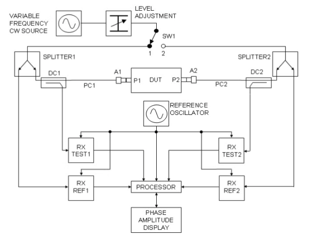
All of the complex receiver output signals are fed to a processor which does the mathematical processing and displays the chosen parameters and format on the phase and amplitude display.

The instantaneous value of phase includes both the temporal and spatial parts, but the former is removed by virtue of using 2 test channels, one as a reference and the other for measurement.

When SW1 is set to position 2, the test signals are applied to P2, the reference is measured by RX REF2, reflections from P2 are coupled off by DC2 and measured by RX TEST2 and signals leaving P1 are coupled off by DC1 and measured by RX TEST1. This position is appropriate for measuring S22 and S12.

NanoVNA

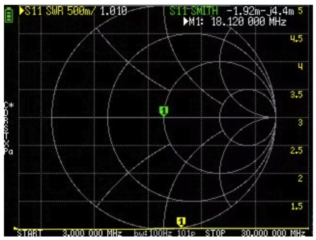
The above graphic represents a Smith chart representation from a NanoVNA device featuring S-parameters on two traces, trace 1 in SWR representation format, and trace 3 for Smith chart representation on R + LC representation.

Overall layout

• Smith Chart (center of screen):
  The big circular grid, with concentric circles and diagonal curves, is a standard Smith chart. It plots the complex reflection coefficient Γ (or normalized impedance) of whatever is connected to Port 1, as you sweep frequency.
• SWR Scale (right‐hand side):
  The yellow numerals 1.5, 2, 2.5, 3, 3.5, 4, 4.5 along the right edge are the VSWR (Voltage Standing Wave Ratio) scale. Although the Smith‐chart grid does not directly show VSWR, many NanoVNAs superimpose both a Smith chart and a side scale that tells you “if Γ lies on a given constant‐circle, that corresponds to X:1 VSWR.”
• Frequency Axis (bottom):
  At the very bottom you see “START 3.000 000 MHz” on the left and “STOP 30.000 000 MHz” on the right. That means the VNA is sweeping from 3 MHz up to 30 MHz.

What’s being measured

• ► S11 SWR 500 mΩ 1.010 (top left):
  In the top‐left corner, the text “► S11 SWR 500 mΩ 1.010” tells you:
  1. We are looking at Port 1’s reflection (S₁₁).
  2. The vertical axis (if you were looking at a traditional dB plot) would be SWR—i.e. the VNA is computing VSWR/Return‐Loss from that reflection coefficient.
  3. “500 mΩ” is simply the impedance reference resolution (i.e. 0.5 milliohm granularity) used for the SWR calculation.
  4. “1.010” is the minimum SWR value seen anywhere in the 3–30 MHz sweep. In other words, this antenna or load is nearly perfectly matched (close to 1 :1) at its best frequency.
• “S11-SMITH –1.92 m + j4.4 m ► M1: 18.120 000 MHz” (top right):
  On the Smith‐chart display (in green), you see the instantaneous complex reflection coefficient at the marker (“M1”) location.
  • “–1.92 m + j4.4 m” means Γ (the complex reflection) at that frequency is about –0.00192 + j0.0044 (i.e. –0.192% real, +0.44% imaginary). Since those numbers are milliscale (“m” = milli), the load is extremely close to the gain‐center of the Smith chart (the perfect 50 Ω point).
  • “► M1: 18.120 000 MHz” tells you that the marker (Marker 1) is sitting at 18.120 MHz. Wherever the little green “1” is on the Smith chart, that is the exact reflection coefficient at 18.120 MHz.

Reading the Smith Chart

• Center of the chart = Perfect match (50 Ω, Γ = 0):
  On a Smith chart, the very center (where the horizontal axis crosses the vertical axis of the outermost circle) represents a normalized impedance of 1 + j0 (i.e. exactly 50 Ω real, no reactance). If your load is exactly 50 Ω, its reflection coefficient is zero and it plots at the very center.
• Where Is “Marker 1”?
  In the picture, Marker 1 (the small green “1” inside a shield) is nearly on the center point of the Smith chart. That corresponds to the numerical readout “–1.92 m + j4.4 m,” meaning at 18.120 MHz the load is almost exactly 50 Ω (just a few thousandths of a unit away).
• Circles & arcs on the chart:
  • The concentric circles around the center are constant‐|Γ| circles. A circle with |Γ| = 0.2, 0.5, 0.8, etc., maps to different SWR values.
  • The diagonal/curved grid lines overlay represent constant‐resistance (vertical lines) or constant‐reactance (arched lines) loci if you were reading the normalized impedance directly.

The SWR curve (overlayed)

Although you’re looking at a Smith chart at the same time, the NanoVNA is also computing VSWR for each frequency and mapping it to the numeric scale on the right (1.5, 2.0, 2.5, 3.0, etc.). If you were watching an S11(dB) or SWR‐vs‐frequency plot, you’d see how the SWR rises above 1.0 as you move away from the best frequency. In this case:

• Because the marker reads “1.010” (in the top‐left), that means the best‐case SWR in the entire 3–30 MHz sweep was 1.01 :1.
• If you traced along the Smith chart from 3 MHz all the way to 30 MHz, you would see the reflection coefficient move around (forming that “loop” you see on the outer portions of the chart). Wherever it falls onto one of those constant‐|Γ| circles corresponds to a specific SWR value on the right‐hand scale.

Interpreting the results

1. Marker location (18.120 MHz):
   • The fact that the reflection point is nearly dead‐center (–0.00192 + j0.0044) means the load (antenna or whatever is attached) is almost exactly 50 Ω resistive, with almost zero reactance, at 18.120 MHz.
   • In practical terms: at 18.120 MHz, VSWR ≈ 1.01, which is essentially a perfect match.
2. Impedance behavior over frequency:
   • If you look at the larger loop on the Smith chart (extending out toward the rightmost edge), that tells you how the normalized impedance moves as you sweep from 3 MHz up to 30 MHz.
   • Where that loop crosses farther away from the center, the SWR is higher (for example, if |Γ|=0.5 at some frequency, that corresponds to about 3:1 SWR on the right scale).
3. Bandwidth & matching:
   • Because the minimum SWR is 1.01 at 18.12 MHz, you know the tuner or antenna is extremely well‐matched there. If you mentally trace out where that loop wanders to |Γ|=0.2 (about SWR = 1.5) or |Γ|=0.333 (SWR ≈ 2:1), you can estimate the usable bandwidth.
   • In other words, any point on the Smith chart that lies inside the circle of radius |Γ|=0.333 (which corresponds to SWR=2:1) is considered “acceptable” for many transceivers. You would note at what frequencies the trace exits that circle, and that gives you your 2:1 bandwidth.

Summary of what you see

• A one‐port reflection (S₁₁) sweep from 3 MHz to 30 MHz is being plotted.
• The Smith‐chart grid is showing how the normalized impedance moves with frequency (i.e. how Γ(f) loops around).
• Marker 1 is placed at 18.120 MHz and reads a nearly perfect match (–0.00192 + j0.0044), corresponding to VSWR = 1.010.
• The yellow SWR scale on the right shows you that at that center point, SWR is essentially 1:1, and as the loop deviates from center you can read off 1.5:1, 2:1, 2.5:1, 3:1, etc.

In practical terms, this display tells you:

“At 18.120 MHz, the device under test is almost exactly 50 Ω resistive (perfectly matched). If you sweep down to 3 MHz or up toward 30 MHz, the match gets progressively worse (Γ moves away from the center), and you can use the SWR scale on the right to see what that VSWR value would be at any point on that loop.”

Key Takeaways:

1. Smith Chart = Complex Reflection (Γ) over frequency.
2. Marker Info (“–1.92 m + j4.4 m @ 18.120 MHz”) = nearly perfect 50 Ω match there.
3. SWR Scale on Right = tells you what VSWR each constant‐|Γ| circle corresponds to.
4. “1.010” (top left) = best SWR seen anywhere in the sweep.
5. Frequency Sweep runs from 3 MHz (left) to 30 MHz (right).

That’s what’s on the screen: a one‐port S₁₁ sweep displayed simultaneously as a Smith chart and an SWR readout, with a marker placed at 18.120 MHz showing an almost ideal match.

Calibration

Calibration is essential to obtain accurate measurements. All RF test setups have some inherent errors: mismatches in cables, imperfect connectors, and device internal offsets. By performing a proper calibration, the NanoVNA characterizes and removes these errors before measuring your Device Under Test (DUT).

Calibration standards

A proper VNA calibration requires three known standards for each port:

1. Open (an open-circuit standard—no load attached).
2. Short (a short circuit).
3. Load (a precision 50 Ω termination, typically with a ±0.1 dB accuracy).

The NanoVNA calibration kit usually includes three SMA adapters: one open circuit, one short (an SMA cap), and one 50 Ω load. If your kit did not include them, you can purchase a calibrated 50 Ω termination and shorting cap separately, but be aware that lower-quality standards can degrade your final measurement accuracy.

One-port vs. Two-port calibration

• One-Port Calibration (S11 only) calibrates Port 1 for reflection measurements. Use this if you only need antenna SWR or reflection coefficient.
• Two-Port Calibration (S11, S21, S12, S22) calibrates both ports. This is necessary when you want to measure insertion loss or transmission through filters, cables, or multi-port devices.

Most amateurs begin with one-port calibration on Port 1 to check antenna resonant frequency and SWR.

One-port calibration procedure (Port 1)

1. Connect the open standard to Port 1
   • On the NanoVNA, go to “Menu → Calibration → Cal1 (Port 1).”
   • Select “Open.” The NanoVNA will measure the open standard at multiple frequencies across your sweep (e.g., 1 MHz to 500 MHz).
   • When it finishes, the screen prompts you to attach the next standard.
2. Connect the short standard to Port 1
   • Choose “Short” from the menu. The NanoVNA measures the short-circuit response.
3. Connect the load (50 Ω) to Port 1
   • Select “Load.” The NanoVNA measures the matched load.
4. Save calibration
   • After loading, the VNA stores the calibration coefficients internally. You can name the calibration (e.g., “Cal Port1 OnePort”) and save it to one of the NanoVNA’s memory slots (typically “Cal 1”, “Cal 2”, etc.).

When complete, the NanoVNA is now calibrated for reflection (S11) on Port 1. If you wish to perform two-port calibration (S11, S21, S12, S22), repeat the same steps on Port 2 (connect the same three standards to Port 2 under “Cal2 (Port 2)”), then perform a “Thru” measurement (connect Port 1 directly to Port 2 with a precision RF jumper for a “through” standard). This extra step references the transmission path.

Tips for better calibration

• Use Clean, Tight Connections: Any dust, loose torque, or bent pins introduce extra mismatch.
• Torque Wrenches or Tightening Tools: Consistent torque (≈ 0.6 Nm) ensures reproducibility.
• Avoid Excess Cable Movement: Once calibrated, try not to flex the NanoVNA’s cables or rig the entire setup in a way that distorts the orientation of the device.
• Re-Calibrate Periodically: If you change cables, move the NanoVNA significantly, or suspect temperature drift, re-calibrate before critical measurements.

Making measurements

With calibration complete, you can now measure S-parameters of antennas, filters, cables, and more. This section focuses primarily on antenna measurements (S11, SWR, and impedance).

Setting up the frequency sweep

1. Define start and stop frequencies
   • Press the encoder knob to enter the “Start/Stop” menu.
   • Dial to set the start frequency (e.g., 1.8 MHz for 160 m band).
   • Press to confirm, then set the stop frequency (e.g., 54 MHz to cover 6 m).
   • Press to return to the main measurement screen.
2. Select trace type
   • There are multiple traces (Trace 1, Trace 2, Trace 3, etc.) that you can assign different measurement displays to.
   • Press and scroll to “Trace 1 → Type → S11 (dB)” for a reflection coefficient in dB.
   • Assign “Trace 2 → Smith” to view a Smith chart of Port 1’s impedance vs. frequency.
   • You can also use “Trace 3 → SWR” if you prefer seeing VSWR directly.
3. Set marker(s)
   • Turning the knob toggles through markers on the active trace.
   • Move the marker along your frequency sweep to identify resonant dips (minimum S11) or match points (e.g., where SWR crosses below 2:1).

Measuring an antenna’s S11

1. Connect the antenna
   • Attach your antenna’s feedline (SMA or via an adapter) directly to Port 1.
   • Ensure the feedline is reasonably short (≤ 1 m) or, if using a longer feedline, you may see feedline effects; you might then want to de-embed the feedline length (advanced).
2. Observe the trace
   • On the “S11 (dB)” display, a good antenna will show a deep notch (e.g., < –10 dB) at its resonant frequency.
   • On the Smith chart, the impedance will move toward the center (50 Ω) at resonance. If it lies on the lower side of the chart (capacitive), you need to add inductance (coil or loading). If on the upper side (inductive), you’d add capacitance (e.g., a hat or more length).
3. Record results
   • Press the knob to freeze (hold) the current display if you want to read the exact S11 and frequency at your marker.
   • The NanoVNA will show the marker’s frequency and S11 in dB, phase, and real/imag parts (depending on trace settings).
4. Save screenshots or data (Optional)
   • If you connect the NanoVNA to a PC via USB and run PC software (e.g., NanoVNA-Saver), you can capture screenshots, save S11 vs. frequency as a CSV, or control the NanoVNA remotely.
   • This is especially helpful for plotting multiple antennas or tracking changes during a tuning process.

Advanced usage and features

Beyond basic antenna SWR testing, the NanoVNA can be used for many advanced tasks.

Measuring transmission (S21)

• Filters and attenuators: Connect Port 1 to the input of a filter, Port 2 to the output. Sweep through the filter’s passband to see insertion loss (S21) vs. frequency.
• Cable loss: Connect a known length of coax between Ports 1 and 2. Measure S21; you can calculate cable attenuation (dB/m) at different frequencies.
• Balun/Transformer testing: Use fixtures to measure how well balanced lines are transformed into unbalanced, by comparing input impedance.

To perform S21:

1. Select a Two-port calibration so that the VNA knows the thru path reference.
2. Set trace 1 → S21 (dB).
3. Place the DUT between Port 1 and Port 2.
4. Observe the insertion loss curve: A well-designed filter will show a deep stopband and a gentle passband slope.

Tips and tricks

• Minimize cable length: You can calibrate using a short precision jumper (< 15 cm) attached to Port 1 alone, then swap directly to your antenna. This yields more accurate SWR readings compared to a long feedline.
• Watch out for harmonics: The NanoVNA’s internal LO can generate harmonics; avoid interpreting spurious spikes. If you see odd notches well outside your antenna band, they may be measurement artifacts.
• Use proper grounding: Place the NanoVNA on a non-conductive surface; avoid touching the board or screen during measurements. Human body capacitance can shift readings slightly.
• Temperature effects: If you take your NanoVNA outdoors in extreme cold or heat, let it stabilize for a few minutes. Drift can cause slight calibration errors.
• Marker math: Many firmware versions allow you to use marker-to-marker delta (Δ) to see bandwidth or frequency shift between two points (e.g., where S11 crosses –10 dB). Utilize this for quick bandwidth measurements.

Conclusion

The NanoVNA has revolutionized the way many amateur radio operators approach antenna tuning and RF measurements. For under $100 (or equivalent in other currencies), you gain a powerful instrument that, although not as feature-rich as professional VNAs, is more than capable of most ham radio tasks:

• Antenna tuning & resonance: Quickly identify resonant points, SWR dips, and match to 50 Ω.
• Filter characterization: Measure insertion loss, passband ripple, and rejection.
• Cable loss measurements: Determine coax performance and detect potential faults.
• Impedance analysis: Use the Smith chart to understand real and reactive components of any DUT.

By mastering calibration and learning to interpret traces (S11, S21, SWR, Smith), you’ll be well on your way to designing better antennas, troubleshooting RF circuits, and gaining a deeper appreciation for how transmission lines behave. As with any tool, practice is key—so calibrate, measure, and experiment with your NanoVNA until you’re confident. Happy measuring!